AlphaThe Surfalize web app is in active development. Features, the user interface and computed results may change at any time, and this documentation may lag behind the app.
Surfalize user guide
Surfalize is a browser-based surface-topography analyser. It loads measurement files from most common profilometers and microscopes, lets you preprocess them with a chain of non-destructive operators, and computes the full ISO 25178 areal and ISO 21920 profile parameter sets, entirely inside your browser. This guide explains how the app is put together and how to use each part. What the parameters themselves mean, with their definitions and formulas, is in the separate parameter reference. For a quick, hands-on introduction, open Help ▸ Guided tour in the app.
Overview
Surfalize is powered by a pure-JavaScript port of the open-source surfalize library. Every computation (loading, levelling, filtering, spectra and parameters) runs client-side. There is no server and nothing to install.
The engine uses 64-bit-addressed typed arrays, streaming algorithms and a background Web Worker, so it comfortably handles very large height maps (tens of megapixels) that would exhaust a conventional in-browser tool.
Getting started
index.html directly.File ▸ Load file…. See supported formats.Analysis group.
A new session auto-runs the guided tour once. You can replay it any time
from Help ▸ Guided tour, and run the interactive
example analysis (a full pipeline on a synthetic surface) from
Help ▸ Example analysis.
The interface
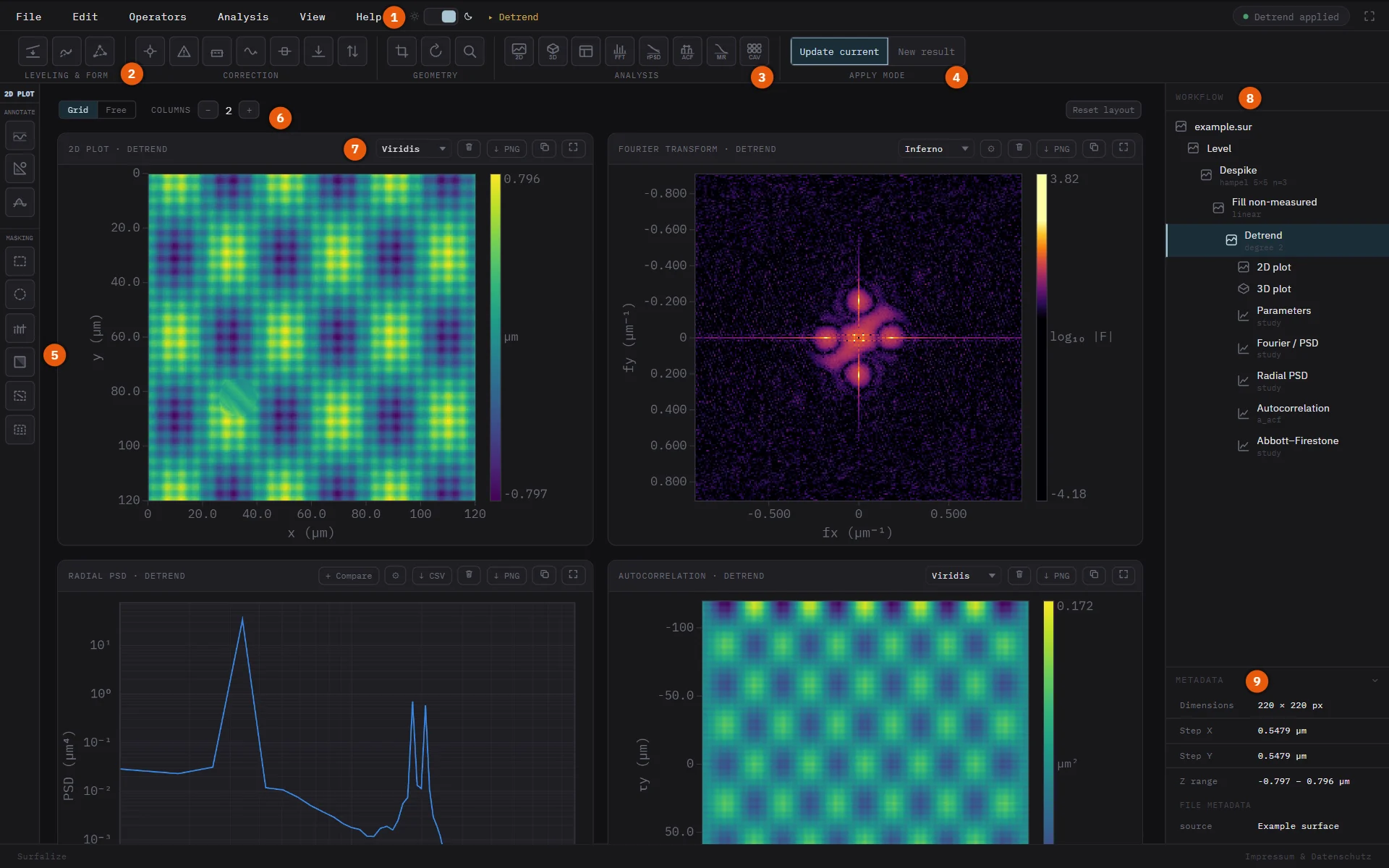
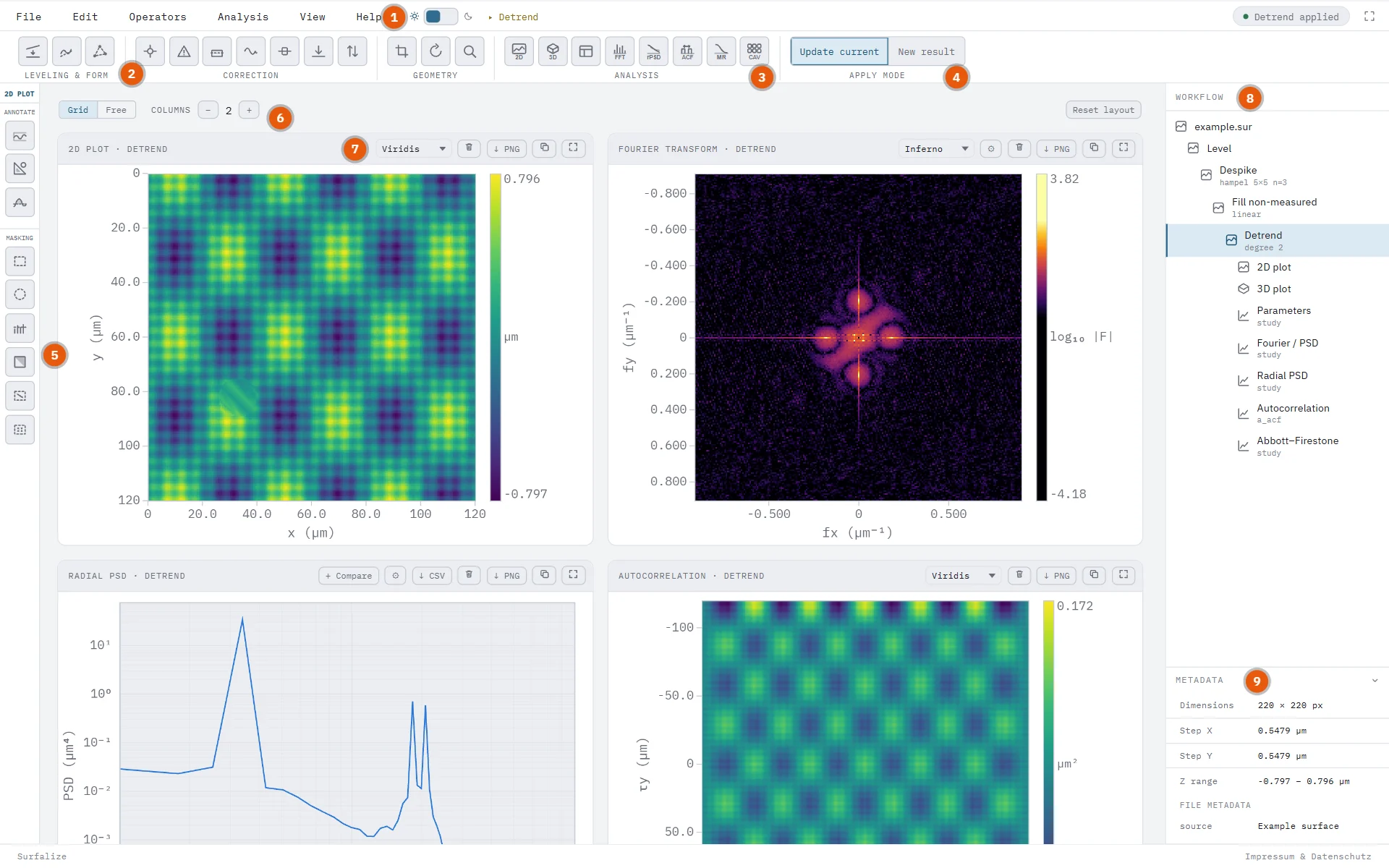
- Menu bar. File, Edit, Operators, Analysis, View and Help. Operators and Analysis repeat the ribbon. The sun/moon switch changes the theme, and the status pill on the right shows what the engine is doing. Edit has Undo (Ctrl+Z), Redo (Ctrl+Shift+Z) and Delete (Del) for the selected node.
- Ribbon: operators. The groups Levelling & form, Correction and Geometry hold the operators. Each one transforms the height data and creates a new state in the work tree.
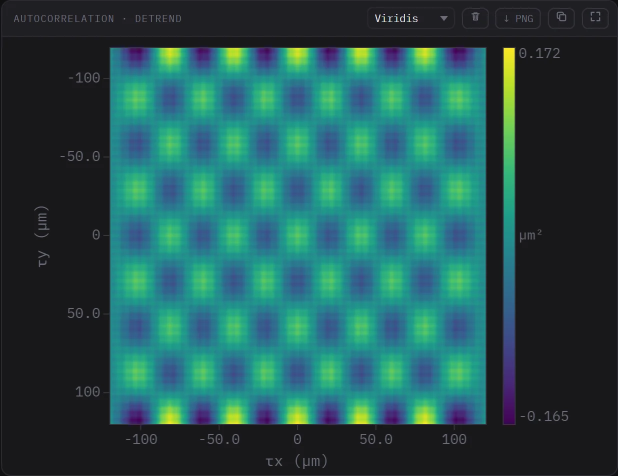
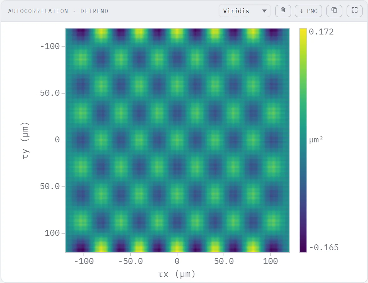
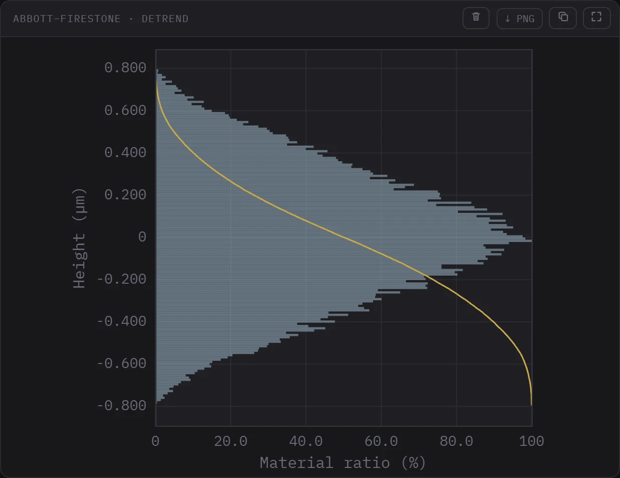
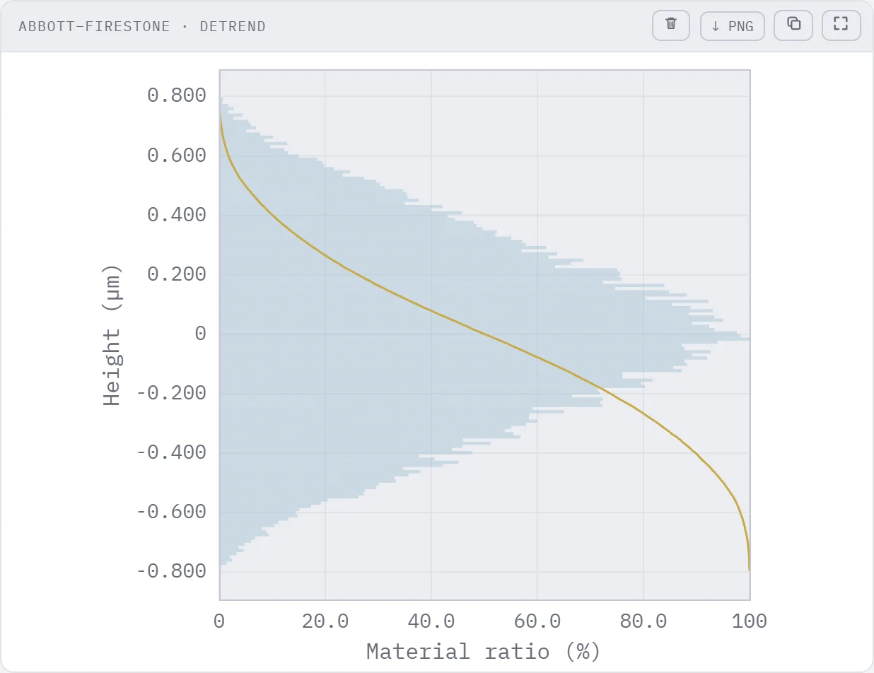
- Ribbon: analysis. Adds views and studies of the selected state: 2D / 3D plot, parameters, spectra, autocorrelation, Abbott curve and cavities. They never change the data.
- Apply mode. Update current or New result: where an operator's result goes. See apply modes; it is worth understanding before you start.
- Tool rail. Tools that annotate a surface without transforming it (Extract, Measure, Construct, Volume), plus the Masking operators.
- Viewport toolbar. The Grid | Free layout switch, the column count and Reset layout. See Layout.
- Panels. Every plot and study is a panel you can move and resize. Several files and several views can be shown at once.
- Work tree. The Workflow panel, the branching history of every state and view.
- Metadata. Dimensions, pixel step, height range and the file's own metadata for the focused surface, in a dock you can collapse.
The work tree
The work tree (the Workflow panel on the right) is the heart of Surfalize: it records every state of your data and every view of it, and it is where you change, branch and reuse a processing.
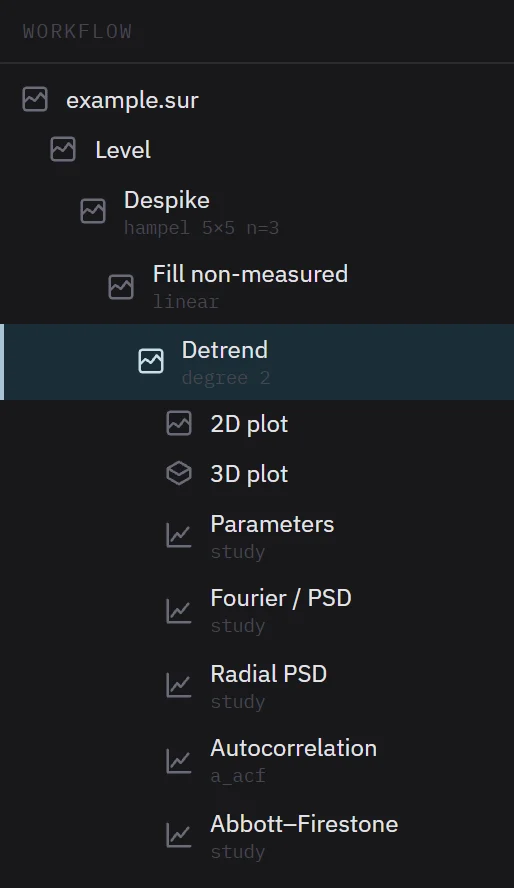
Reading the tree
Apply modes: Update current vs New result
Operators never overwrite data: every operator creates a new state, and the state it started from is kept. The apply mode, the Update current New result switch on the right of the ribbon, decides where the new state goes and what happens to the panels you already have open.
The figures show both modes on the same starting point. A levelled, despiked and filled surface has a 2D plot and a parameter table, and a high-pass filter (λc = 25 µm) is applied to the Fill non-measured state.
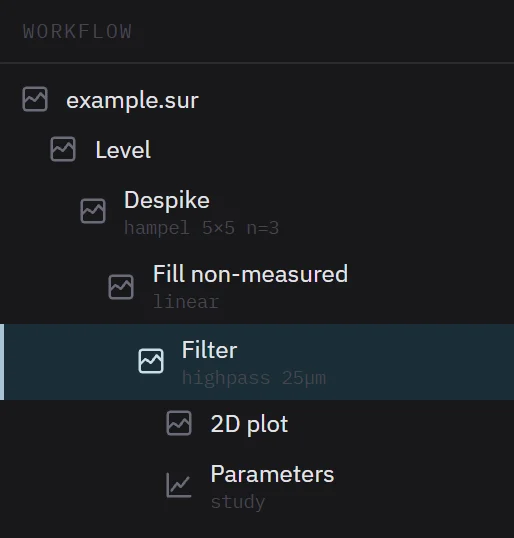
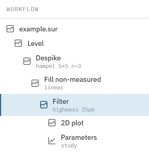
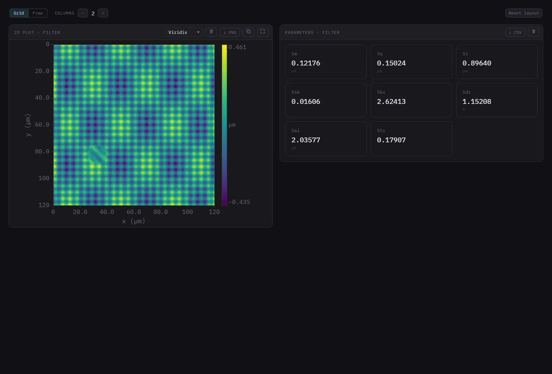
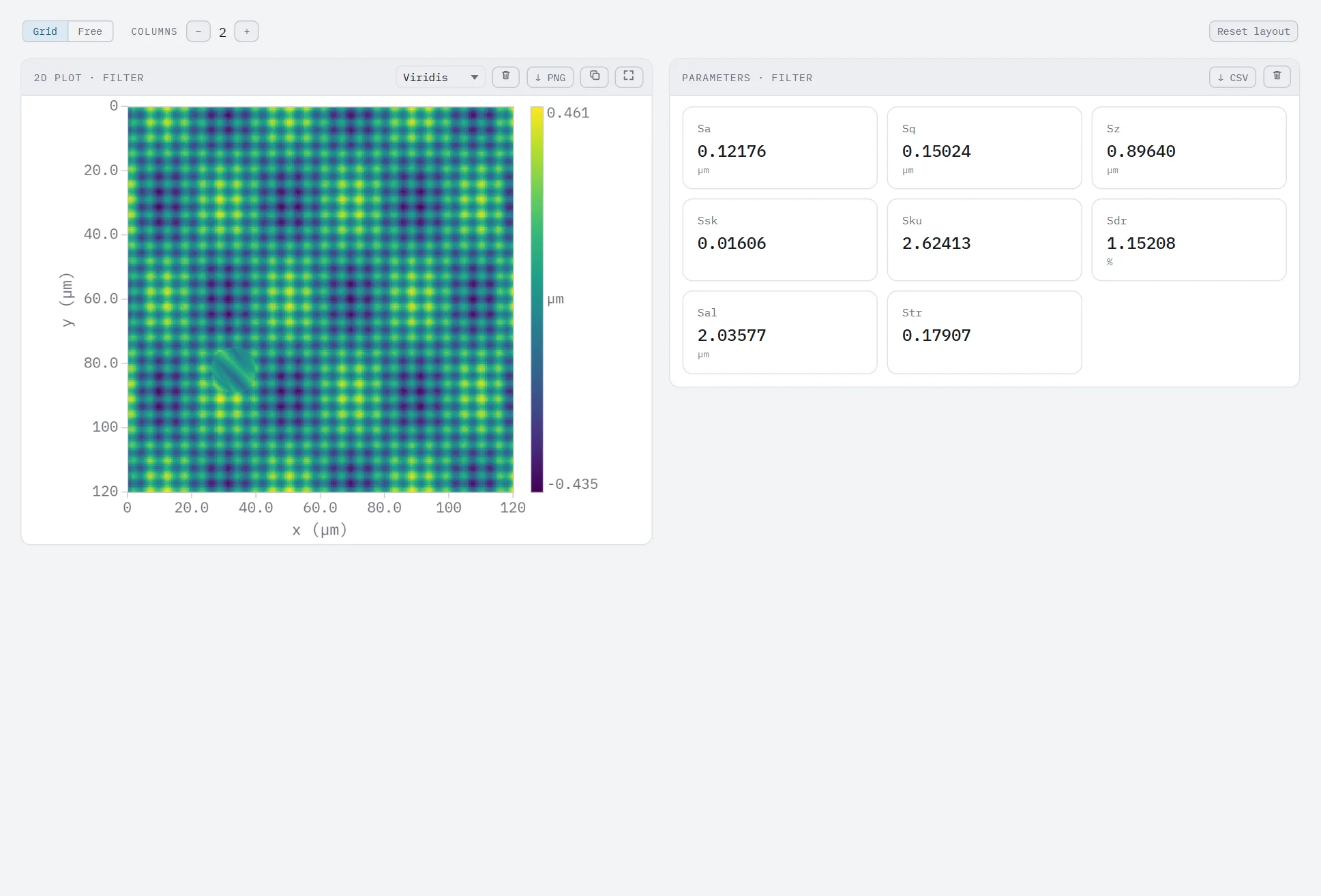
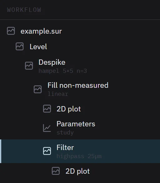
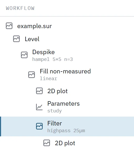
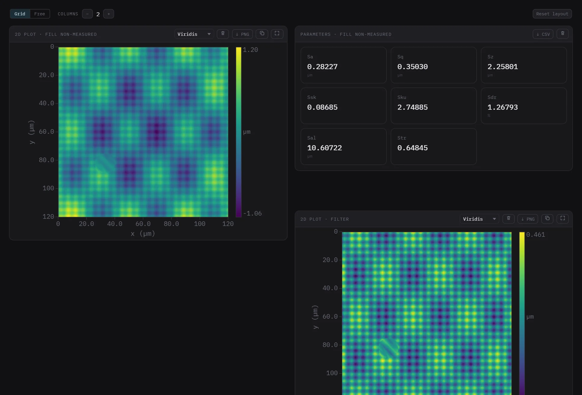
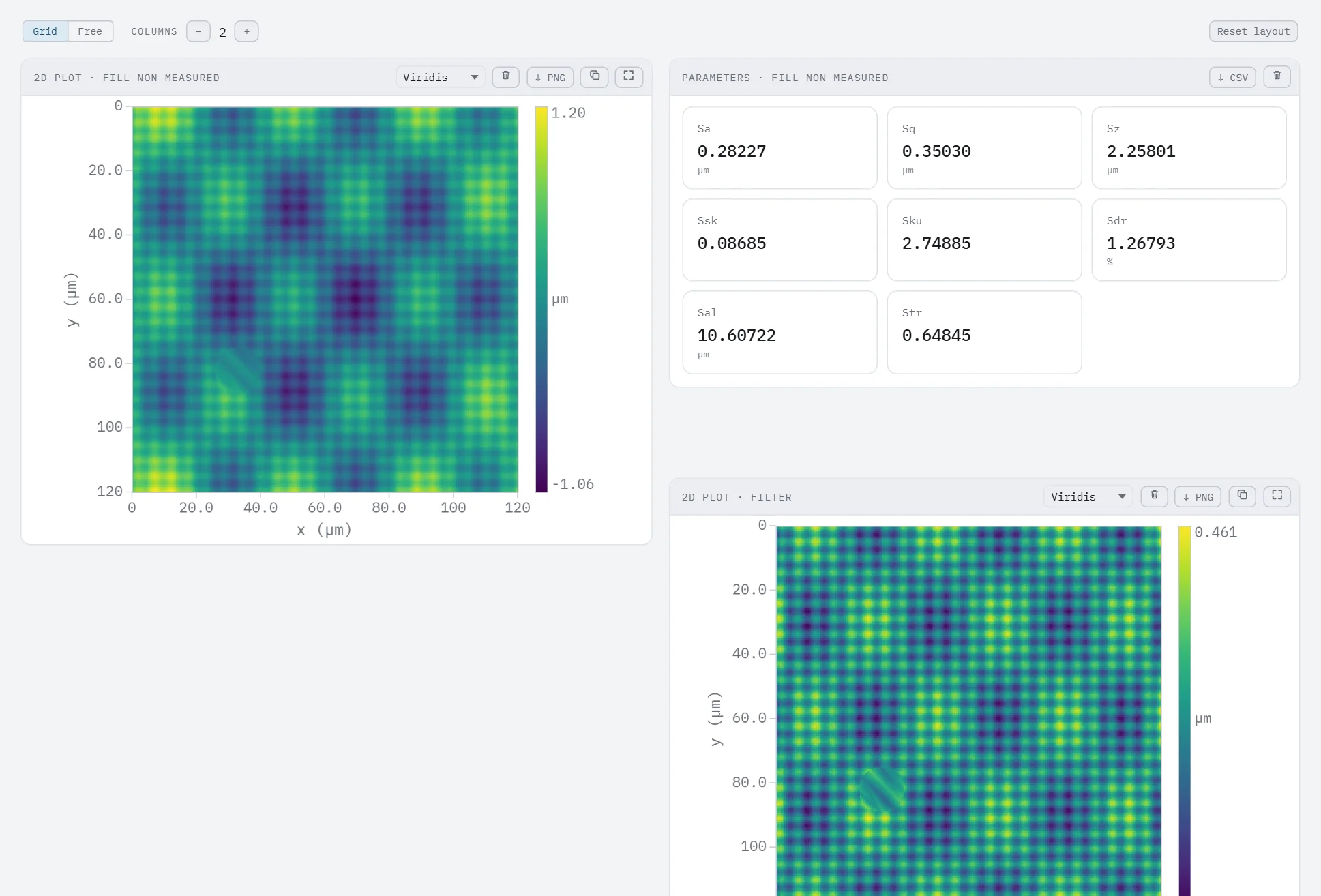
You can switch modes at any time; the choice is remembered. A branch created with New result can later be dragged onto another state, and a chain built with Update current can still be branched with ⧉ Duplicate (below).
Editing, branching and rearranging
Hover a node to show its buttons:
The Edit menu steps through this history: Undo (Ctrl+Z) and Redo (Ctrl+Shift+Z) reverse or replay operators, deletions and other work-tree changes, and Delete (Del) removes the selected node or panel.
Swapping the measurement
A root has one more button, ⇄Exchange file. It loads a different file into that root and re-runs the whole tree on it: the same operators, analyses and panels, now on the new data. Profile lines you drew are carried over, scaled to the new field. This is the quickest way to apply a finished processing to the next sample. To keep a processing for later, save it as a workflow; to run it on many files at once, use batch processing.
Operators
Operators preprocess the height map. They can be chained in any order, and each one produces a new work-tree state (where it goes depends on the apply mode). Operators with settings open a dialog with a live preview; the others apply at once.


Levelling & form
Correction
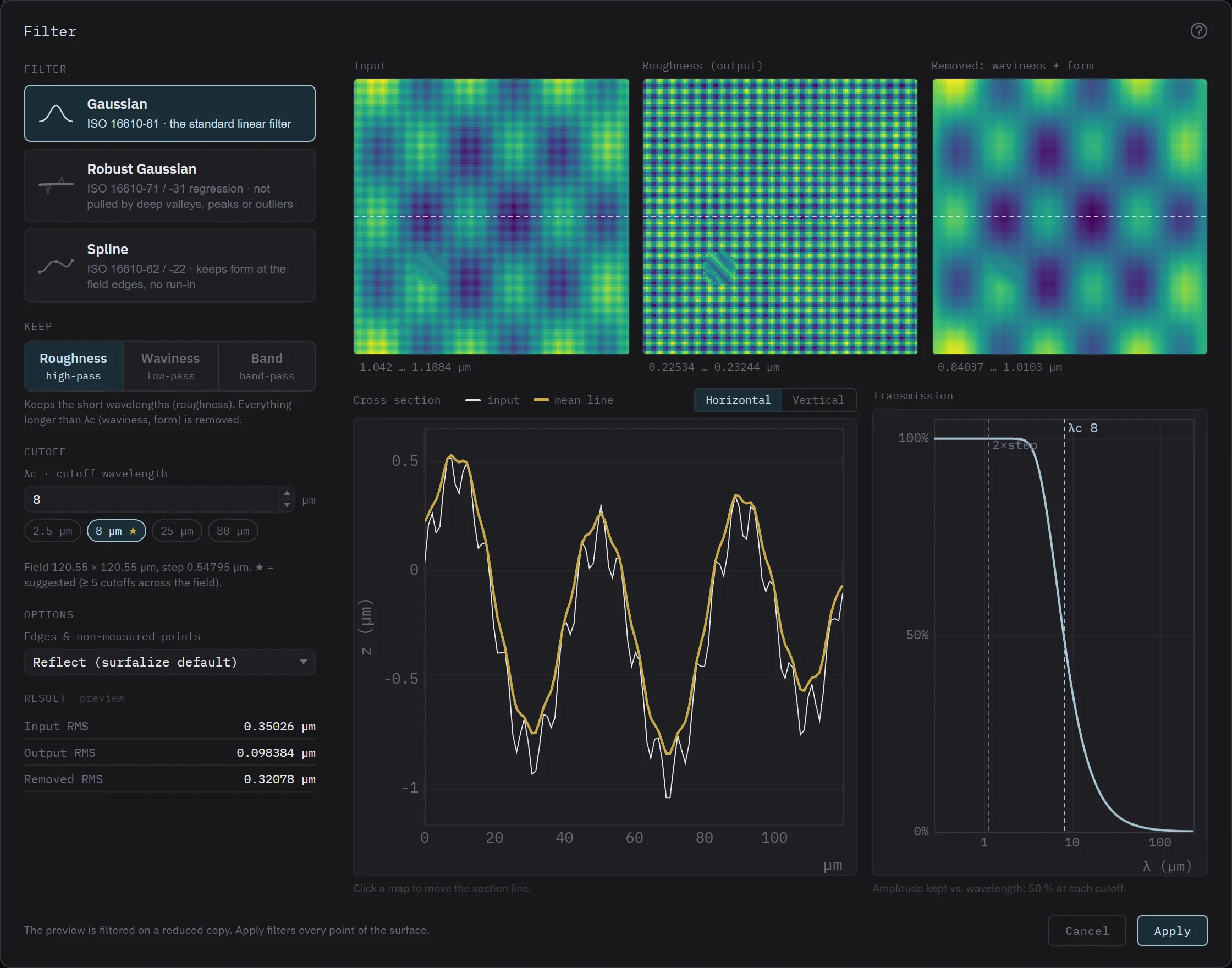
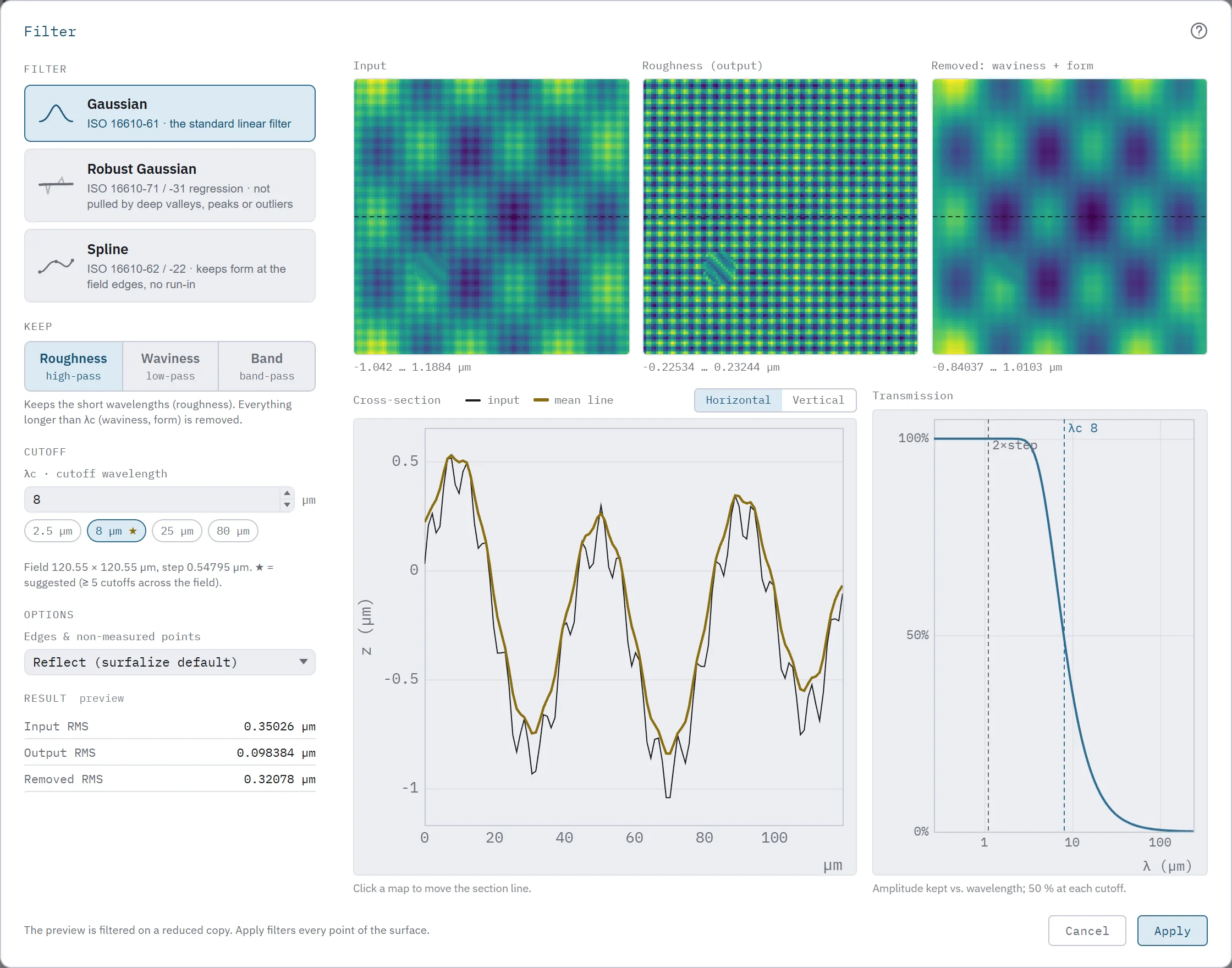
Geometry
Masking on the tool rail
Masks exclude regions from the parameters without deleting the data. They are operators too, so each mask creates a new state.
Analysis panels
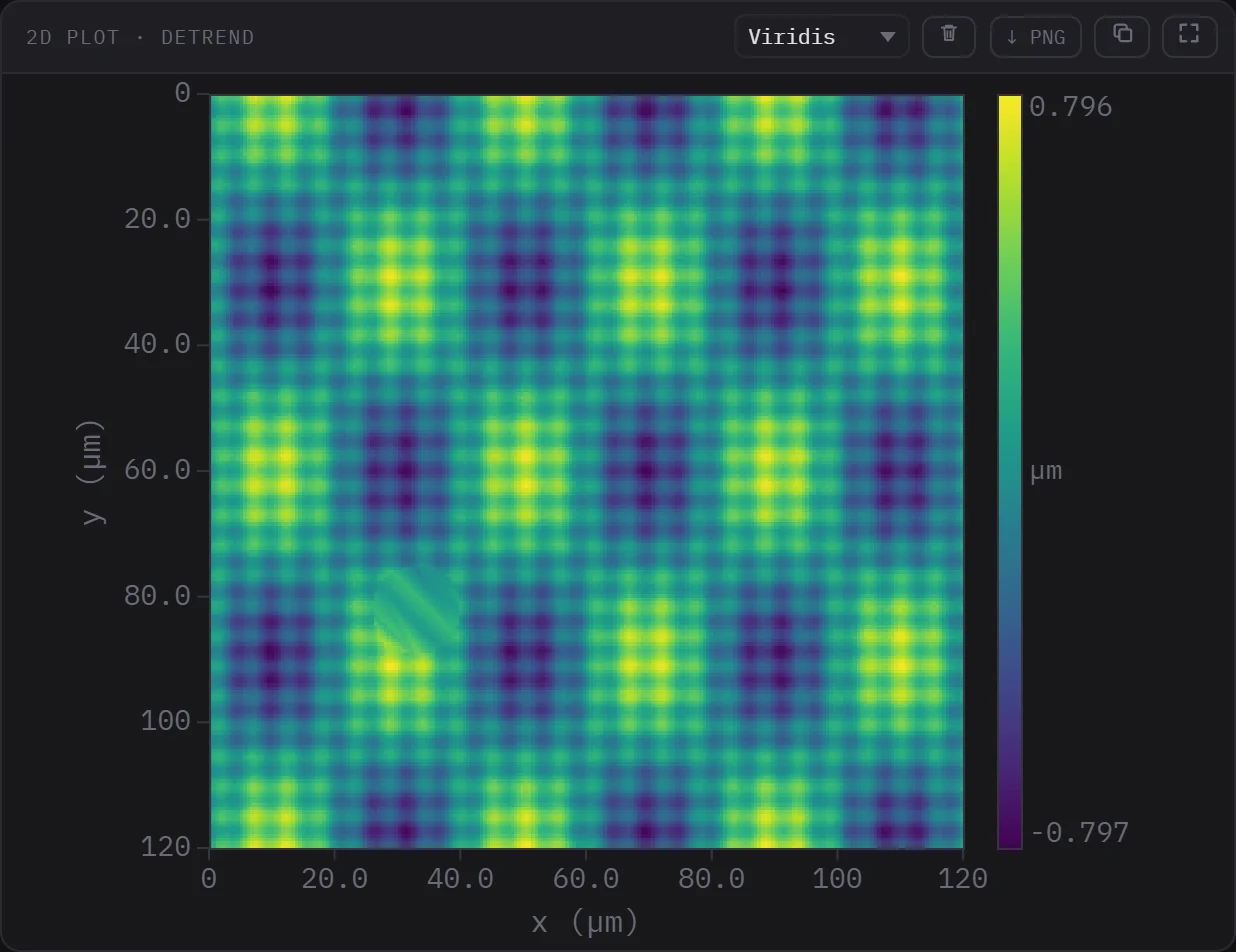
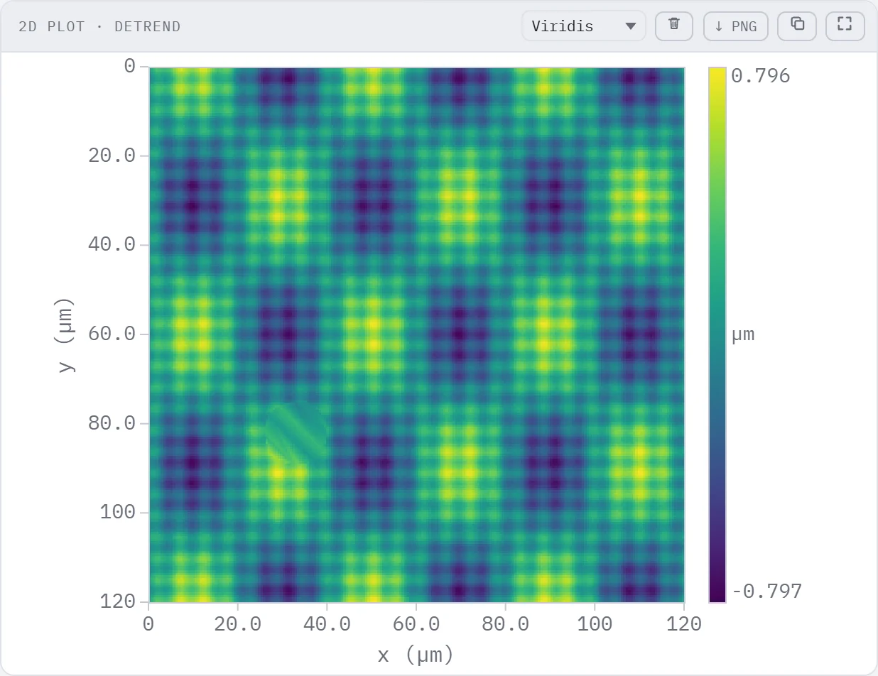
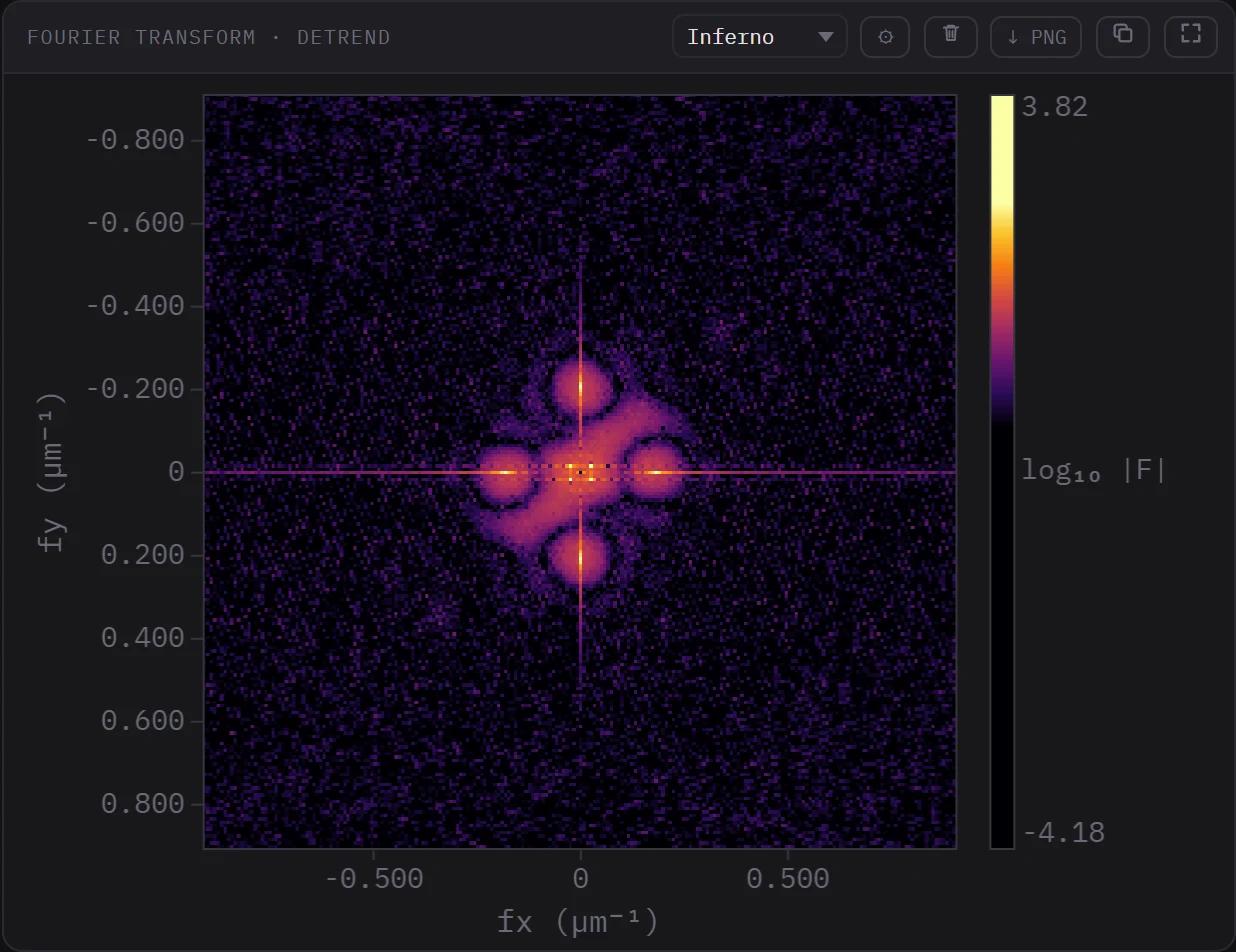
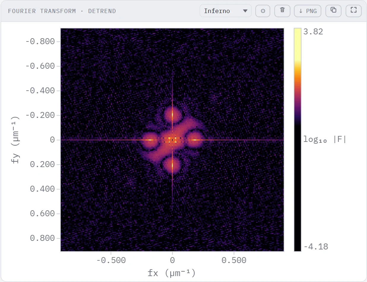
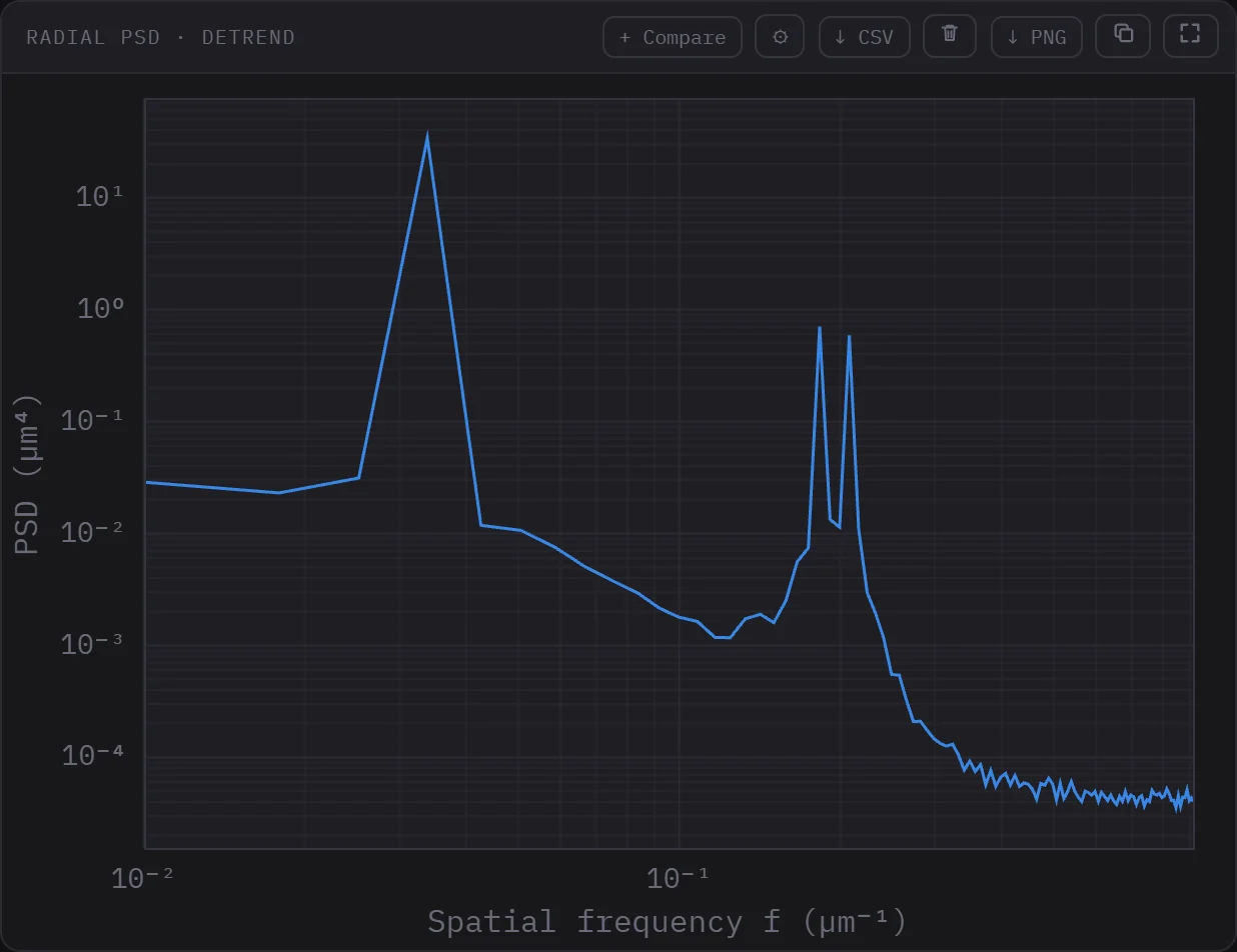
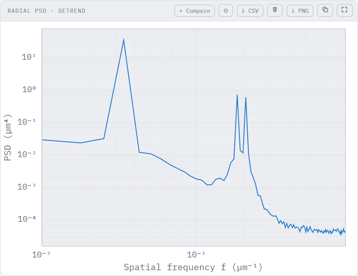
The Analysis group opens views and computations of the selected state as panels in the viewport. They never change the data, and with Update current they follow the state as you add operators. Every panel header has the same buttons: a colormap where it applies, ⚙ settings, remove, ↓ PNG (or CSV) to export, copy to the clipboard, and full screen.
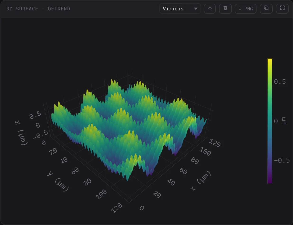
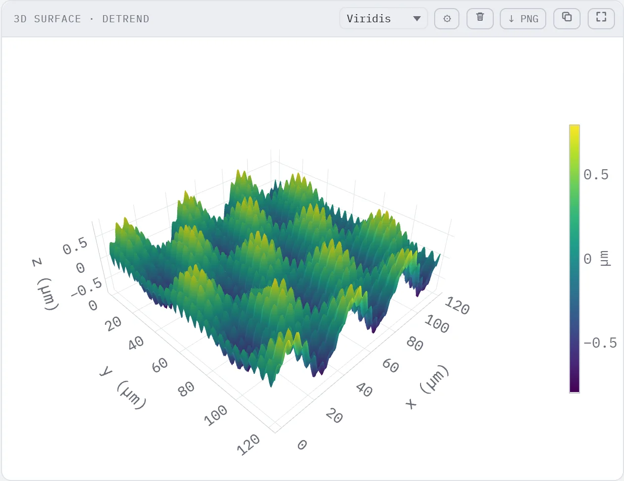
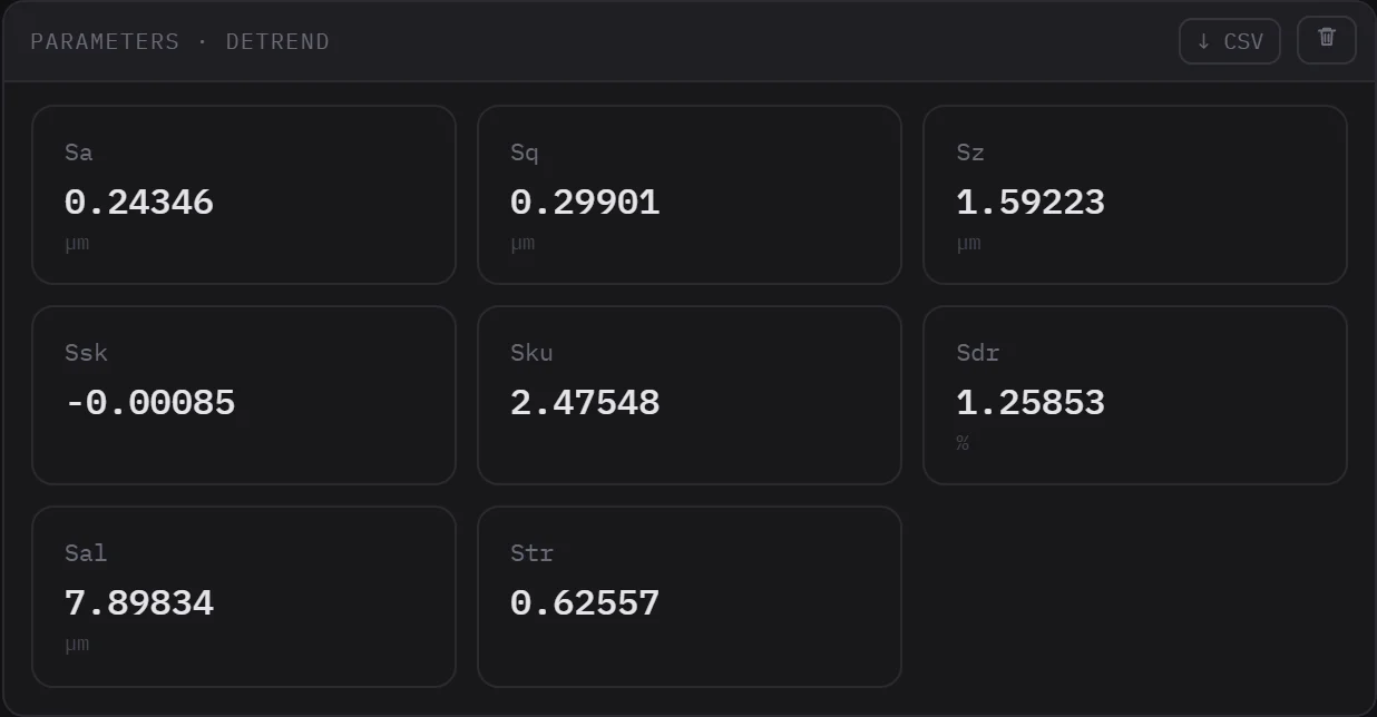
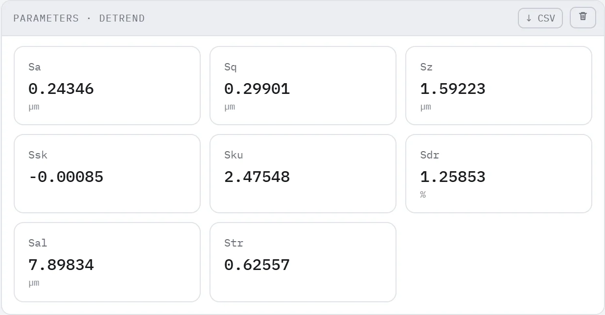
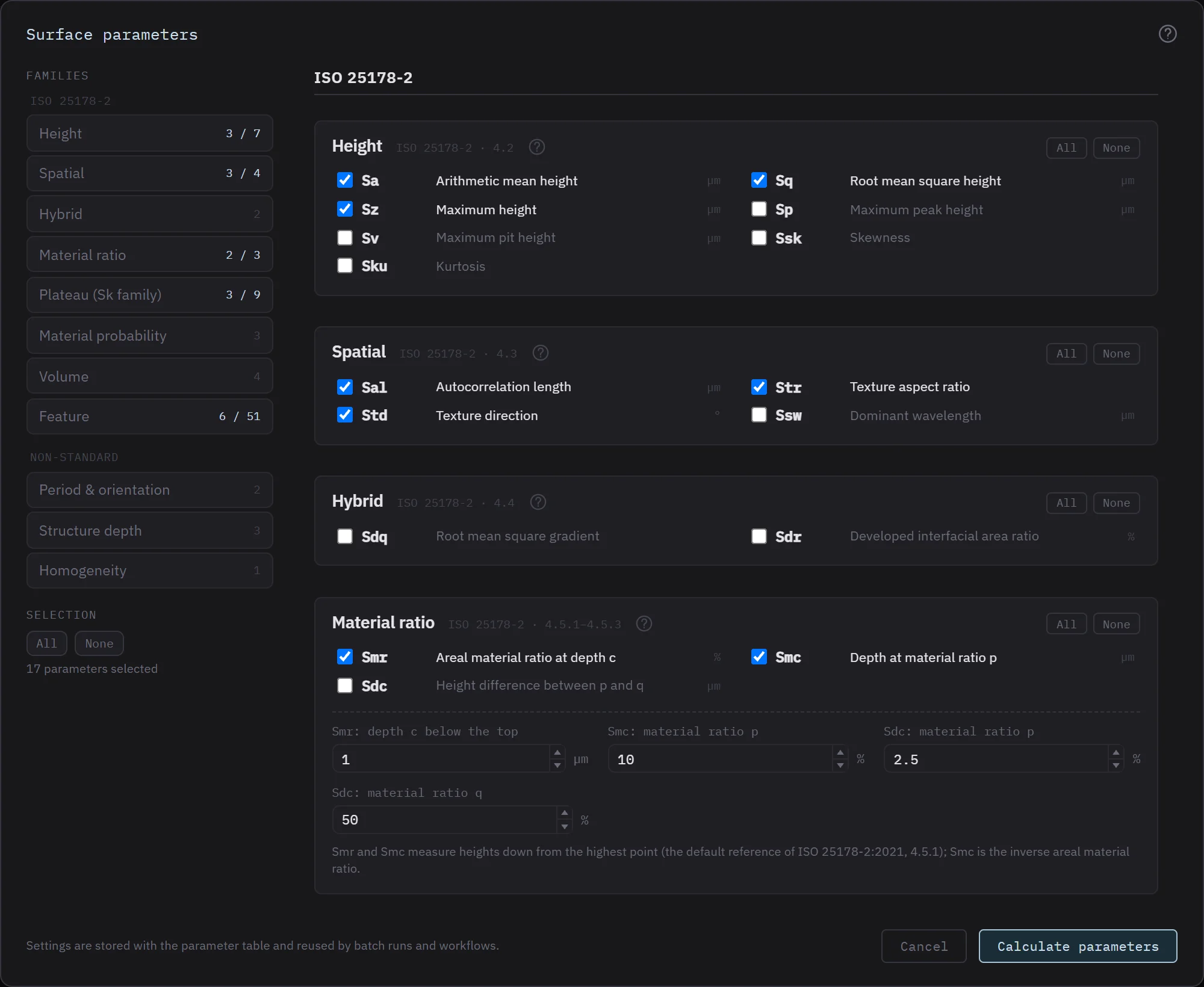
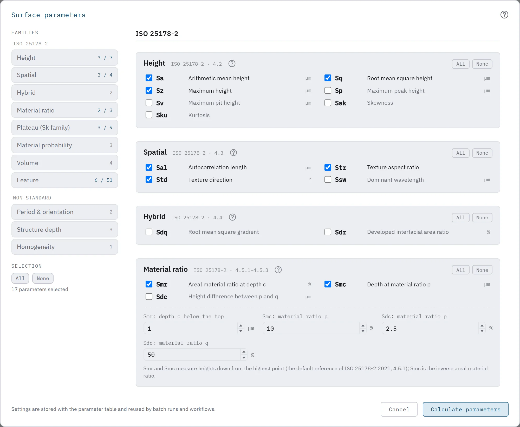
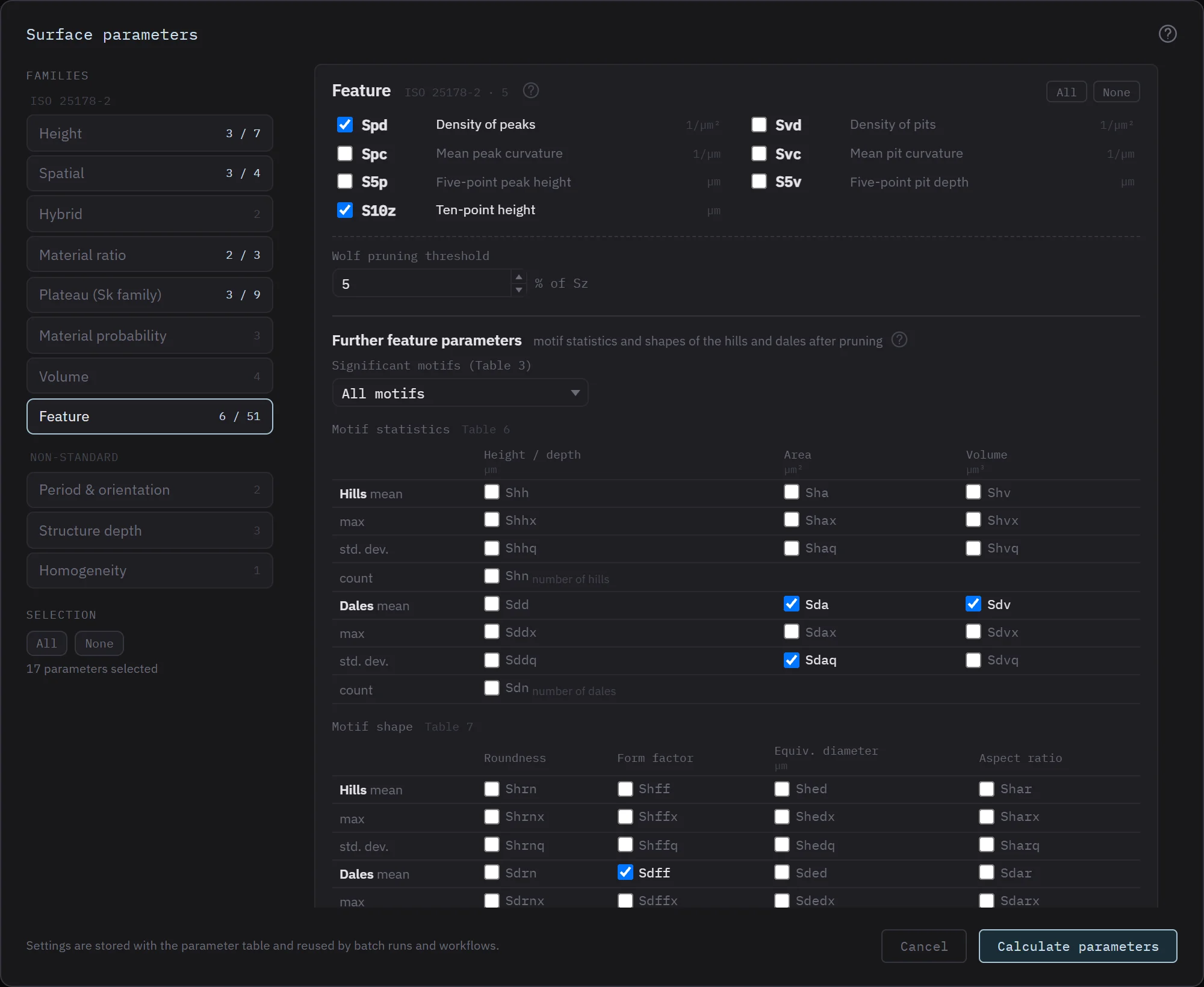
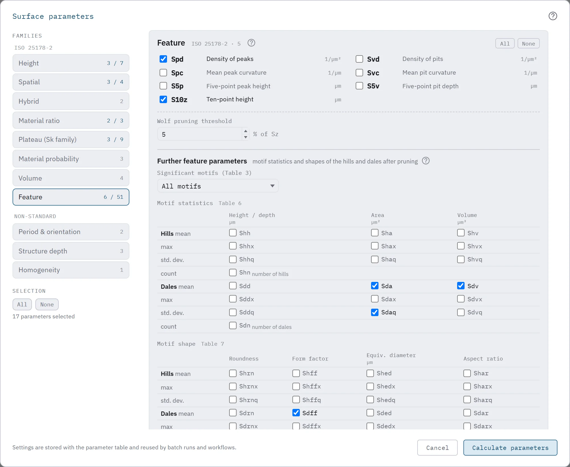
The Parameters dialog lists the parameter families of the standard on the left: height, spatial, hybrid, material ratio, plateau (Sk family), material probability, volume and feature. Each entry shows how many of its parameters are ticked; a click jumps to the family. On the right, every family is a section of its own with its parameters (symbol, name, unit), All / None for that family, and the settings its parameters depend on:
- Material ratio: the depth c for Smr (measured down from the highest point), the ratio p for Smc, and p, q for Sdc.
- Volume: the material ratios p and q (10 % and 80 % by default).
- Feature: the Wolf pruning threshold in % of Sz. Below the seven named feature parameters, Further feature parameters offers the motif statistics of ISO 25178-2 Table 6 (local height or depth, area and volume of the hills and dales, each as mean, maximum or standard deviation, plus their number) and the motif shapes of Table 7 (roundness, form factor, equivalent diameter, aspect ratio) as two hill / dale matrices, with the choice which motifs count: all, or those open or closed at a height given as a material ratio.
The settings are stored with the parameter table, shown under every value that depends on them (and in the CSV), and reused when the table is recomputed, in batch runs and by saved workflows. The pen on a table reopens the dialog with its selection and settings. On a selected profile the dialog shows the profile (R) families of ISO 21920-2 instead.
Tools
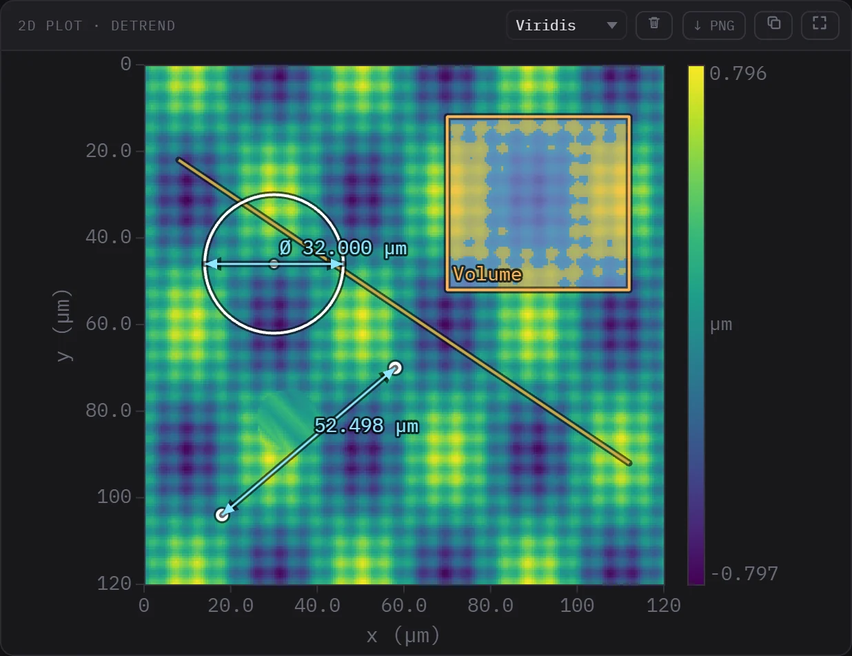
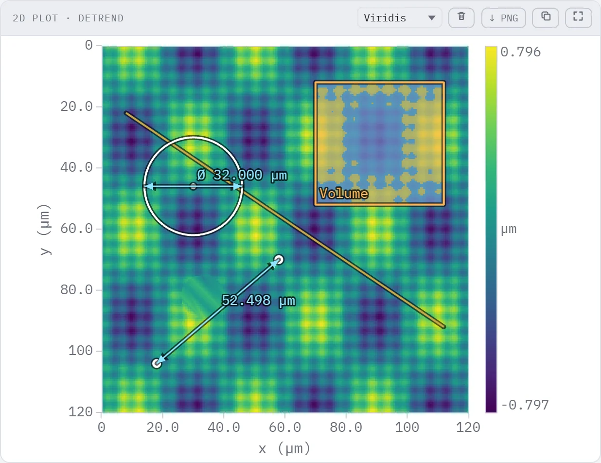
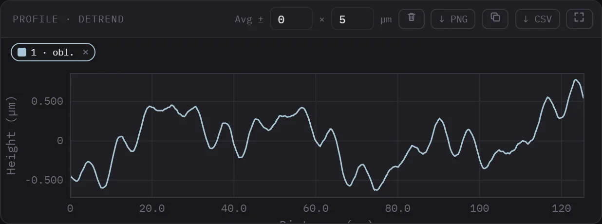
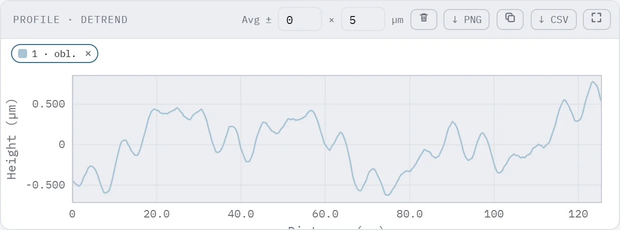
Tools live on the left rail and annotate the focused surface without changing its height data. Pick a tool, then click or drag on the 2D plot; one tool is active at a time. The results get their own panels and work-tree nodes under the surface.
Extract: profiles
Construct, Fit, Find & Measure: geometry metrology
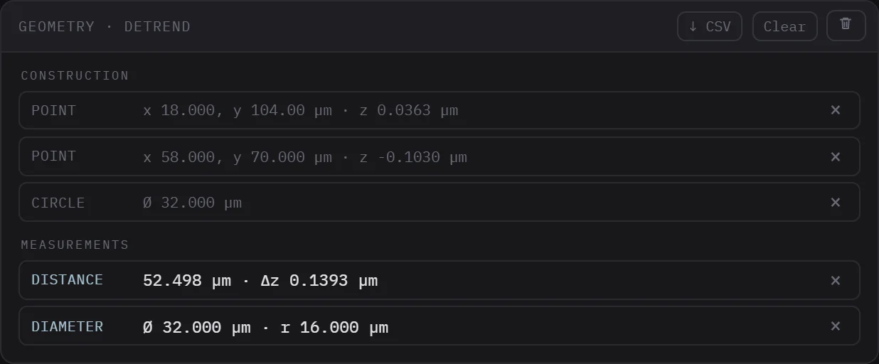
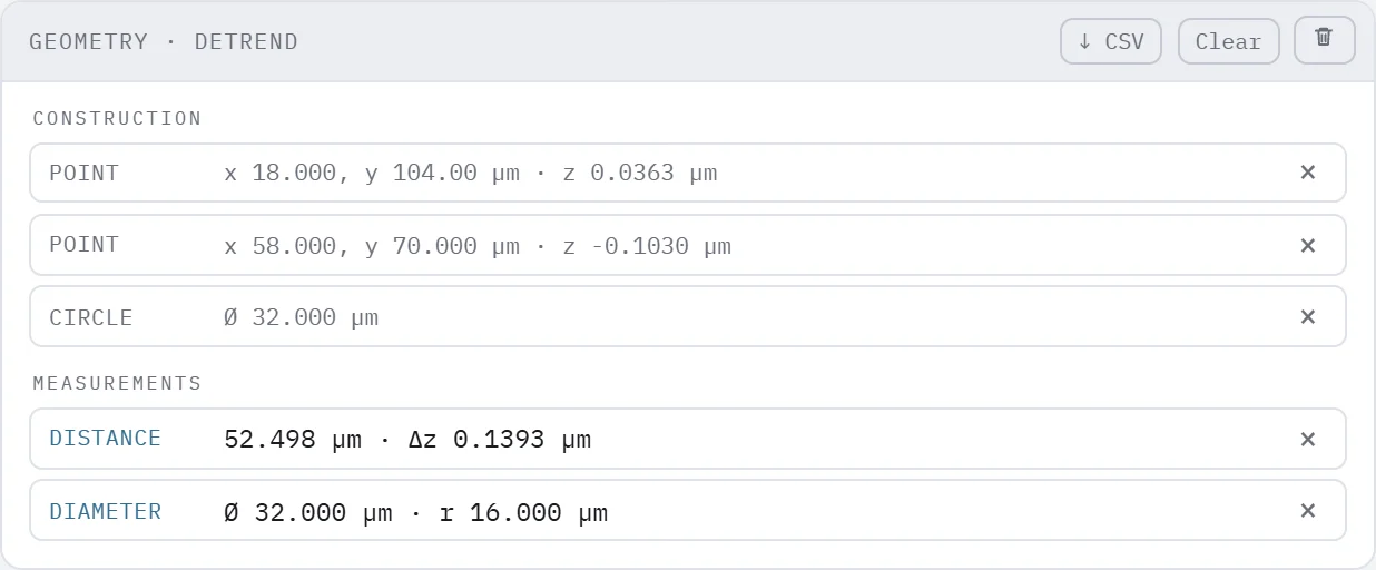
A Geometry panel keeps construction geometry (points, lines, circles and what is built from them) apart from measurements. You first construct or detect the geometry, then dimension it with the Measure tool, as with a smart dimension in CAD. Construction geometry is drawn in white; measurements are drawn as dimensions in light blue.
Construction items can be dragged by their handles or moved as a whole; whatever is built on them and every measurement of them follows. New points snap to the points already on the map (points, line ends, circle centres, feet, intersections, minimum and maximum points), and a ring shows the point a click will land on. A snapped point stays on that point: a line started on a minimum point follows it when you move the minimum’s search box. Drag the point away to release it. The panel lists the construction geometry, then the measurements; removing an item also removes what is built on it and its measurements.
Volume
Batch processing
Open File ▸ Batch… to work over many files at once. There are two modes:
- Analyze & export: replay the current workflow (its operators and selected parameters) across a set of files and export the combined parameter tables as CSV/TSV or an Excel workbook, plus per-panel images. A pinned colour range keeps the images comparable across files.
- Convert format: re-save each input file as a different output format, downloading a single file directly or several as one zip.
Stitching tiles
An area larger than one field of view is often measured as a grid of overlapping tiles.
File ▸ Stitch tiles… puts such tiles back together into one surface. It lines
them up on the texture they share in each overlap, matches their heights and blends the
seams. Tiles are placed to the whole pixel and never resampled, so every measured value
outside the overlaps is kept as it is.
Adding tiles
Click Add files… or drop the tile files on the box. Any supported format
works, but all tiles must have the same pixel size. The list is sorted by name the way
people read numbers, so tile_2 comes before tile_10. Its order is
the scan order: the first entry is tile 1. Use ↑ and
↓ to move a tile, and × to remove it. The tiles stay in
the dialog and are not added to the work tree.
Layout
The layout describes how the instrument scanned the area, and it gives every tile its nominal place:
- Rows and Columns: the size of the grid. They are filled in from the number of tiles until you change them, and the grid needs at least one cell per tile.
- Nominal overlap: how much neighbouring tiles overlap, as a share of the tile size. Use the value set on the instrument (the chips offer common ones).
- Scan order: whether the instrument filled the grid row by row or column by column.
- First tile: the corner where the scan started.
- Meander: tick it when every other row (or column) was scanned in the opposite direction.
If the preview shows a jumbled picture, the layout does not match the scan: check the order, the first tile and the meander option first.
Alignment
- Refine positions by correlation: compares the texture in each overlap and moves the tiles to where it fits best, which corrects stage errors. Untick it to place the tiles exactly on the nominal grid.
- Max. correction: how far a tile may move from its nominal place, as a share of the tile size. Raise it when the stage is known to be imprecise; keep it small on repetitive textures, where a match one period away can look just as good.
- Min. match: the similarity (0 to 1) an overlap must reach to be used. Overlaps below it are rejected and do not move the tiles.
- Height matching: corrects each tile against the others so the heights agree in the overlaps, either by an offset and a tilt, by an offset alone, or not at all.
- Overlap blending: how the overlaps are filled. Linear feathering fades smoothly from one tile to the next and hides the seams best. Average takes the mean of the tiles, and Later tile on top keeps the tile that comes later in the list.
Reading the preview
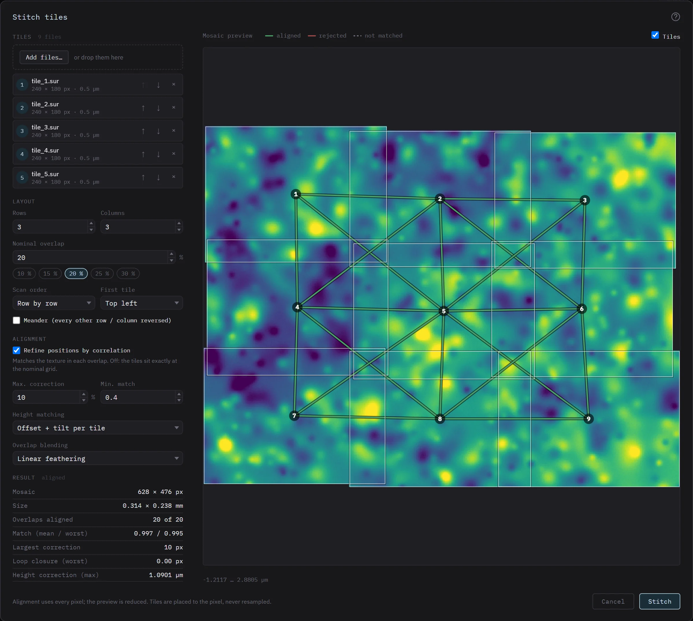
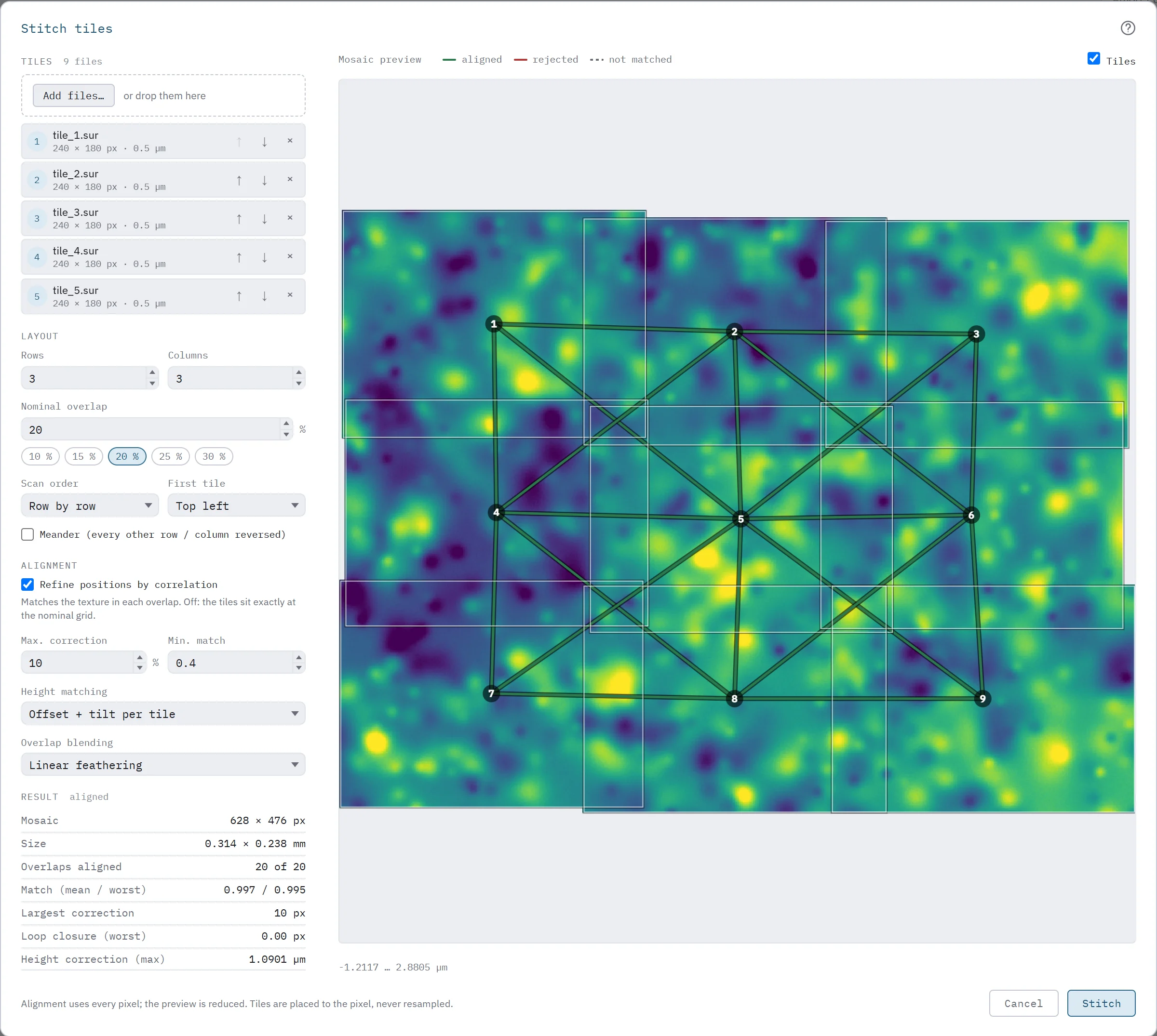
The preview shows the blended mosaic at reduced resolution. It updates as soon as you change a setting: first with the nominal layout, then with the aligned positions once the alignment has run (the state next to Result says which). With Tiles ticked, each tile is outlined and numbered in list order, and a line joins the centres of every pair of tiles that overlap:
- Green: the overlap was matched and used to place the tiles.
- Red: the overlap was rejected, because its match stayed below the minimum or because it disagreed with the other overlaps.
- Dashed: the overlap was not matched, for example because correlation is switched off or no usable match was found.
Hover over the preview to see which tile files lie under the pointer.
The Result read-out sums up the alignment:
- Mosaic and Size: the size of the stitched surface, in pixels and in millimetres.
- Overlaps aligned: how many of the overlaps were used.
- Match (mean / worst): how similar the overlapping tiles are once aligned, on the same 0 to 1 scale as Min. match. Values close to 1 mean the texture fits well.
- Largest correction: the largest distance a tile was moved from its nominal place, in pixels. A value close to the maximum correction is a sign to check that overlap.
- Loop closure (worst): how far, in pixels, the matched overlaps disagree with each other once every tile is placed. A fraction of a pixel means they agree.
- Height correction (max): the largest offset applied by height matching.
- Rejected and Not aligned (highlighted): the rejected overlaps, and the tiles left at their nominal place because none of their overlaps was used.
The stitched surface
Stitch becomes available once the alignment has finished. It blends the
tiles at full resolution and adds the mosaic as a new file in the work tree, named
Mosaic (n tiles), with its own 2D plot. From there it works like any loaded file.
A saved workflow cannot reload the mosaic, because it was never
a file on disk. To reuse it, export it first
(File ▸ Export file…) and load that file with the workflow.
Export & PDF
Export a file
File ▸ Export file… saves any work-tree state (the raw file or any transformed
result) to another format, with per-format options: compression, embedded image layers,
binary/ASCII and comments. Writers are available for .sur, .sflz,
.sdf, .tmd, .al3d and .x3p.
Export the view as PDF
File ▸ Export view as PDF… renders the on-screen panel grid to a multi-page A4
landscape PDF that preserves the layout. Plots are embedded as high-resolution images;
parameter tables, headers and cards stay as selectable vector text. Pages follow the app
theme.
Workflows
A workflow captures your whole session structure (the node tree, every operator and its
parameters, view settings, profiles, geometry items, volume settings and parameter
selections) as a small .surfflow.json file. The topography itself is
not included, so the file stays tiny and shareable.
Save with File ▸ Save workflow…. To restore, use File ▸ Load workflow…
and select the .surfflow.json together with the topography file(s) it
references; Surfalize reloads them and replays every step.
Layout & themes
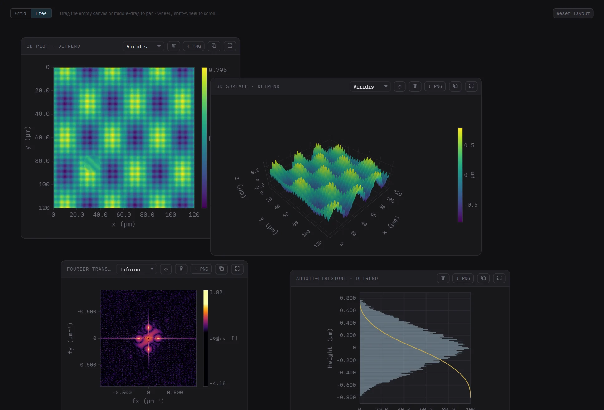
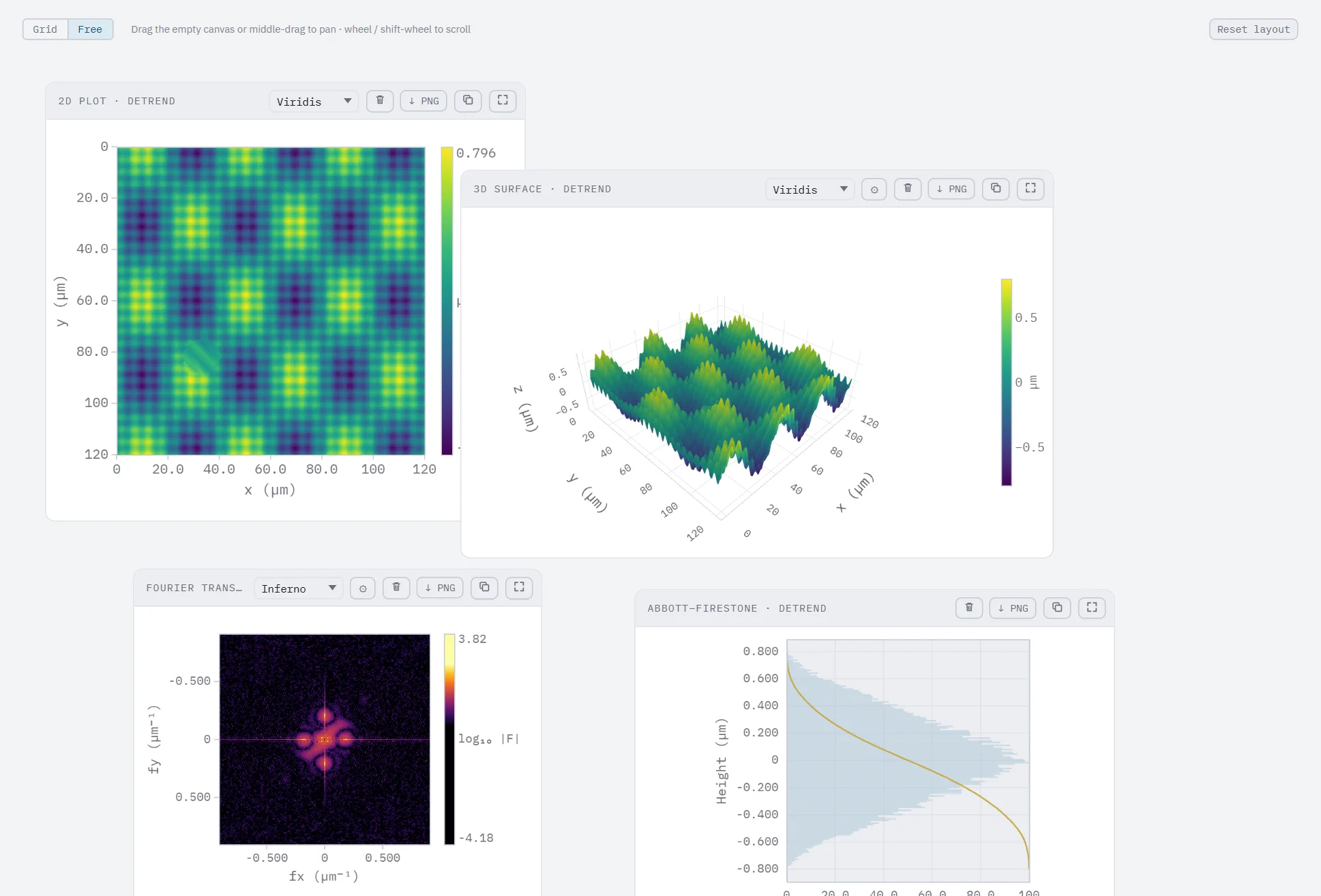
Panels are arranged in one of two layouts, chosen with the
Grid Free switch at the left of the toolbar
above the panels (or View ▸ Layout). Both show the same panels; only the
arrangement differs, and each layout keeps its own arrangement, so you can switch back and
forth without losing either.
Grid
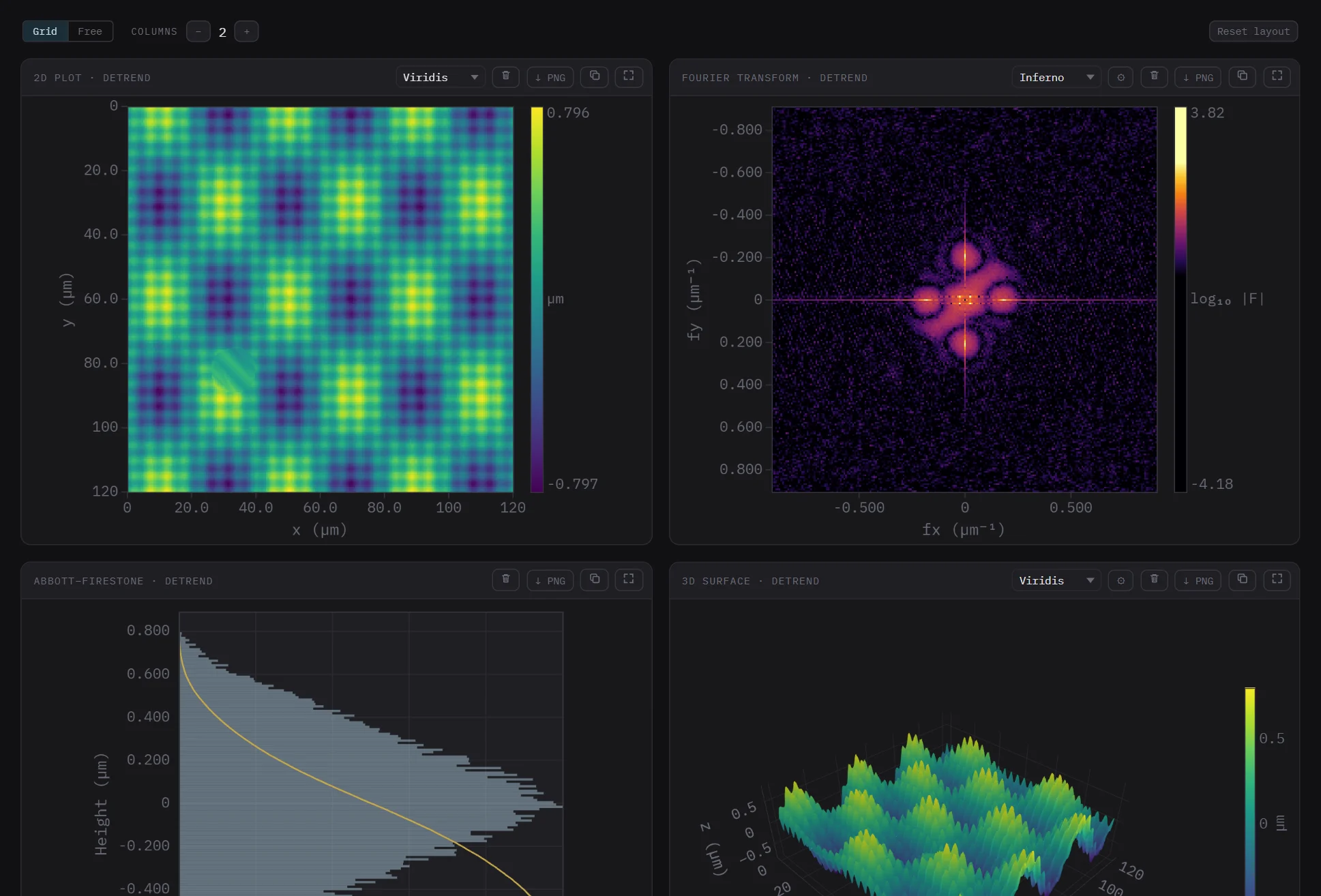
The default. Panels snap to a grid of columns. Drag a panel by its header to move it and by its bottom-right corner to resize it; panels never overlap. The − / + buttons set the number of columns (1–4): fewer columns give each panel more room, more columns show more panels at once. Show grid (View menu) keeps the empty cells visible. Use it when you want a tidy, regular page, for example for a PDF export.
Free canvas
An unbounded whiteboard. Drag panels anywhere by their header and resize them freely from the corner; the panel you click comes to the front. Pan by dragging the empty canvas, with the middle mouse button anywhere, or with the wheel (shift-wheel scrolls sideways). Dragging a panel against the edge of the view scrolls the canvas and extends it. Show grid draws a dot grid. Use it to group panels by meaning (one sample's views together, a comparison next to it) or to make one plot much larger than the rest. The first switch keeps the arrangement you had in the grid.
In both layouts Reset layout returns every panel to its default size and place, and sizes and positions persist between sessions. Export view as PDF keeps the arrangement, splitting pages only between panels.
Themes
Switch between the Dark and Light themes in the
View menu or with the sun/moon switch, which is also on this page and the
validation and legal pages. The choice applies everywhere, including the plots and any other
open Surfalize tab, and is remembered for next time. The figures on this page follow it too.
Supported formats
Read:
Write:
Tips & FAQ
Nothing shows after I load a file
Make sure the file is a supported format and not corrupted. Errors appear in a dialog; the file's metadata (if read) is shown in the Metadata dock.
How do I compare several measurements?
Just load them one after another. Each file gets its own panels in the shared grid; increase the column count in View to see more at once, or use Batch for a table across files.
Are the parameters standard-compliant?
Every areal and profile parameter is validated against reference software to within numerical tolerance (see the validation results). This tool is provided without warranty; verify independently before use in safety-critical work.
Where can I learn more about the maths?
The parameter reference defines every parameter with its formula. The surfalize library documentation covers the underlying algorithms and parameter definitions in detail.